Title: Computational Fluid Dynamics 01: Rectangular grids without for loops Date: 2017-05-03 08:30 Category: ComputationalFluidDynamics Tags: Python, grid generation Slug: cfd-01-rectangular-grid-genereation-python Cover: /p5101/img5101/output_7_0.png Authors: Peter Schuhmacher Summary: Vectorized Python code to generate basic rectangular grids
Aequidistant rectangular grids
When the area of interest can be discretizised by a rectangular aequidistant grid, we do not need explicit variables x and y to define the grid. The mesh sizes dx and dy are sufficient to discretizise the governing equations in this case. With streched and/or curvilinear grids, however, each grid point has to be computed and stored explicitly. In this case a aeqidistant rectangular grid is the starting point and by mapping the streched and/or curvilinear grid is computed.
Algebraic grids
In this section we will consider algebraic grids. Algebraic grid means that the grid can be constructed by closed formulas for the mapping. On the other side are the numerical grids that contain a differential equation that has to be solved numerically. The starting point for each numerical is a algebraic grid however.
Using the outer product to generate grids
The outer product - also called dyadic product - is a matrix multiplication. Better knwon than the outer product is the inner product, also called dot product or scalar product, which is a matrix multiplication too.
For constructing a rectangular grid we need
a 1-dimensional (nx,1)-matrix X containing the locations of the grid points in the x-direction
a 1-dimensional (1,ny)-matrix Y containing the locations of the grid points in the y-direction
an auxilliary matrix onesX with the same dimensions as X but all matrix elements are 1
an auxilliary matrix onesY with the same dimensions as Y but all matrix elements are 1
The x- and y--coordinates for each grid point are given by
A compact Python code for a rectangular grid
In the code we use ix, iy instead of onesX, onesY. This gives the following few lines of code without any for-loop to build a rectangular grid:
import numpy as np
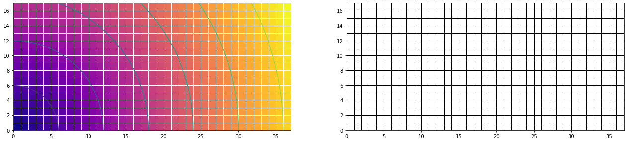
nx = 38; ny = 18
#---- set the 1-dimensional arrays in x- and y-direction
ix = np.linspace(0,nx-1,nx)
iy = np.linspace(0,ny-1,ny)
#---- use the outer product of 2 vectors -----------
x = np.outer(ix,np.ones_like(iy)) # X = ix.T * ones(iy)
y = np.outer(np.ones_like(ix),iy) # Y = ones(ix) * iy.T
plt.pcolormesh()
plt.pcolormesh() has changed its functionality. The dimension of the value parameter (z) must be of lower dimension than the dimesions of the corners (x,y). So we intruduce the helper function redu()-
def redu(A): return A[0:-1,0:-1]
The graphical display
#====  The following is for the grafics ===============
import matplotlib.pyplot as plt
import matplotlib.colors as mclr

z =np.sqrt(x*x + y*y) # set a fancy Z function
z1 = redu(z)
z2 = np.zeros_like(z1)

fig = plt.figure(figsize=(22,11))
ax1 = fig.add_subplot(121)
ax1.pcolormesh(x, y, z1, edgecolors='w',cmap="plasma")
ax1.contour(x, y, z)
ax1.set_aspect('equal')

myCmap = mclr.ListedColormap(['white','white'])
ax4 = fig.add_subplot(122)
ax4.pcolormesh(x, y, z2, edgecolors='k', lw=1, cmap=myCmap)
ax4.set_aspect('equal')
plt.show()