.ipynb .pdf

Binder

Contents

Title: Computational Fluid Dynamics 02: Body-fitted grids without for loops Date: 2017-05-06 08:30 Category: ComputationalFluidDynamics Tags: Python, grid generation Slug: cfd-02-body-fitted-grid-genereation-python Cover: /p5102/img5102/output_7_0.png Authors: Peter Schuhmacher Summary: Vectorized Python code to generate basic rectangular grids

Python code for a terrain-following grid

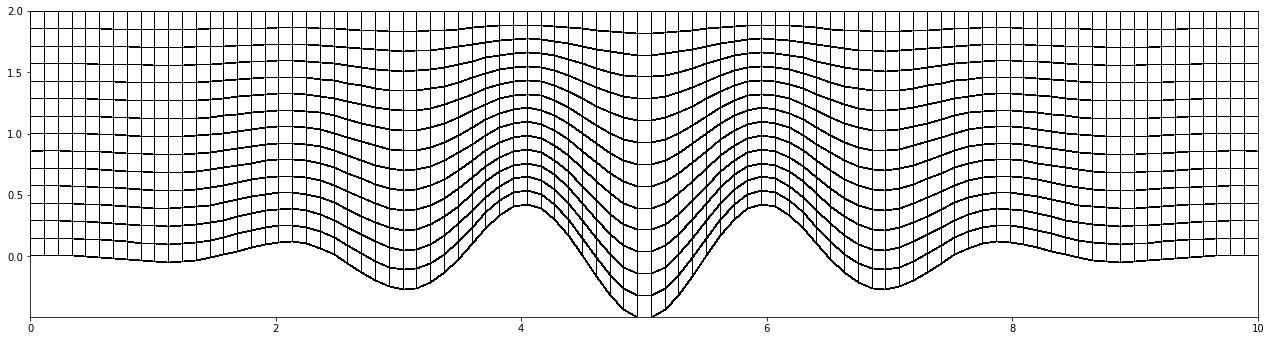
In this example the terrain-followin property is executed in the y-direction. The x-coordinate is determined as in the rectangular case in the previous example. At each x-grid point the y-coordinate is computed as

\[ y = y_{bottom} + \eta \cdot (y_{top} - y_{bottom}) = y_{bottom} + \eta \cdot dY \]

where \(\eta\) varies between 0..1. In the following code iy has the role of \(\eta\) . Again the outer product completes the grid efficiently.

import numpy as np
import matplotlib.pyplot as plt
import matplotlib.colors as mclr

def scale01(z):   #--- transform z to [0 ..1]
    return (z-np.min(z))/(np.max(z)-np.min(z))

def scale11(z):   #--- transform z to [-1 ..1]
    return 2.0*(scale01(z)-0.5)

plt.pcolormesh()

plt.pcolormesh() has changed its functionality. The dimension of the value parameter (z) must be of lower dimension than the dimesions of the corners (x,y). So we intruduce the helper function redu()-

def redu(A): return A[0:-1,0:-1]

import numpy as np

nx, ny = 90, 15
Lx, Ly = 10, 2
ix = np.linspace(0,nx-1,nx)/(nx-1)
iy = np.linspace(0,ny-1,ny)/(ny-1)

#--- set some fancy south boundary ----
A = 0.5; B = 1.0; C = 5.0; D = 0.25
south_boundary = B*np.exp(-(scale11(ix)/A)**2) * D*np.cos(scale01(ix)*C*2.0*np.pi)
north_boundary = np.ones_like(south_boundary)
dY =  north_boundary - south_boundary

#--- generate the GRID: use the outer product to complete the 2D x-/y-coord
x = np.outer(ix,np.ones_like(iy))
y = np.outer(dY,iy) + np.outer(south_boundary,np.ones_like(iy))

#---- grafics ------------------------------------------------
#--- scale for the graphics ---------------
X=x*Lx;  Y=y*Ly

#--- graphical display
fig = plt.figure(figsize=(22,22)) 
myCmap = mclr.ListedColormap(['white','white'])
ax4 = fig.add_subplot(111)
z = redu(np.zeros_like(X))
ax4.pcolormesh(X, Y, z, edgecolors='k', lw=0.75, cmap=myCmap)
ax4.set_aspect('equal')
plt.show()

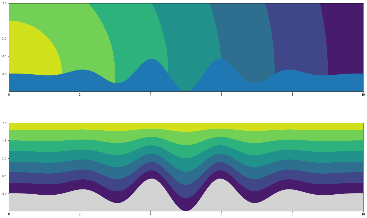
Have some fun

#--- set some fancy Z-values ---------
Z1 = (np.sqrt(X*X + Y*Y))
Z2 = (np.outer(np.ones_like(dY),iy))
Z3 = (Y)

#---- experiment with the graphics --------
fig = plt.figure(figsize=(22,14)) 
ax1 = fig.add_subplot(211)
ax1.contourf(X, Y, -Z1)
ax1.fill_between(ix*Lx, south_boundary*Ly, min(south_boundary)*Ly)
ax1.set_aspect('equal')

ax1 = fig.add_subplot(212)
ax1.contourf(X, Y, Z2)
#ax1.pcolormesh(X, Y, Z2, edgecolors='w',cmap="plasma")
ax1.fill_between(ix*Lx, south_boundary*Ly, min(south_boundary)*Ly,facecolor='lightgrey')
ax1.set_aspect('equal')
plt.show()

\[\]

Python code for a terrain-following polar grid

1. ix has the role of the angle \(\phi\)

2. ix is transformed to sx so that the grid points will be concentrated in the middle of the \(\phi\)-domain

3. iy has the role of the radius \(r\)

4. iy is transformed to sy so that the grid points will be concentrated at the lower boundary of the \(r\)-domain

5. (x,y) is the grid in polar coordinates (\(\phi, r\))

6. (x,y) is transformed to the cartesian coordinates (X,Y)

import numpy as np
import matplotlib.pyplot as plt
import matplotlib.colors as mclr

nx = 38; ny = 18
ix = np.linspace(0,nx-1,nx)/(nx-1)
iy = np.linspace(0,ny-1,ny)/(ny-1)

#---- stretching in x- = angular-direction ---------
ixx =  np.linspace(0,nx-2,nx-1)/(nx-2)
dxmin = 0.1;                                # minimal distance as control parameter
dxx = 1.0-np.sin(ixx*np.pi) + dxmin         # model the distances
sx = np.array([0])                          # set the starting point
sx = scale01(np.cumsum(np.append(sx,dxx)))  # append the distances and sum up

#---- stretching in y- = radial-direction ---------
yStretch = 0.5; yOffset = 2.95                    # control parameters
sy = scale01(np.exp((yStretch*(yOffset+iy))**2)); # exp-stretching

#---- complete as polar coordinates --------------
tx = np.pi * sx            # use ix as angel phi
ty =   1.0 + sy            # use iy as radius r [1.0 .. 2.0]

x = np.outer(tx,np.ones_like(ty))  
y = np.outer(np.ones_like(tx),ty)  

#---- transform to cartesian coordinates ---------
X = y * np.cos(x) # transform to cartesian x-coord
Y = y * np.sin(x) # transform to cartesian y-coord

The graphical display

#---- grafics---------------------------------------------
fig = plt.figure(figsize=(22,11)) 
ax1 = fig.add_subplot(221)
ax1.contourf(X, Y, x + y)

ax2 = fig.add_subplot(222)
c1, c2 = np.meshgrid(iy*(ny-1),ix*(nx-1))
myCmap = mclr.ListedColormap(['blue','lightgreen'])
z2 = redu((-1)**(c1+c2))
ax2.pcolormesh(X, Y, z2, edgecolors='w', lw=0.75, cmap=myCmap)

myCmap = mclr.ListedColormap(['white','white'])
ax3 = fig.add_subplot(223)
z3 = redu( np.zeros_like(X))
ax3.pcolormesh(X, Y, z3, edgecolors='k', lw=0.5, cmap=myCmap, alpha=0.5)
ax3.contourf(X, Y, X+Y, alpha=0.75)

ax4 = fig.add_subplot(224)
ax4.pcolormesh(X, Y, redu(0*X), edgecolors='k', lw=1, cmap=myCmap)
plt.show()

Aequidistant rectangular grids Types and test cases in 2-dimensional space